24 Improving performance
Attaching the needed libraries:
24.1 Exercises 24.3.1
Q1. What are faster alternatives to lm()? Which are specifically designed to work with larger datasets?
A1. Faster alternatives to lm() can be found by visiting CRAN Task View: High-Performance and Parallel Computing with R page.
Here are some of the available options:
speedglm::speedlm()(for large datasets)biglm::biglm()(specifically designed for data too large to fit in memory)RcppEigen::fastLm()(using theEigenlinear algebra library)
High performances can be obtained with these packages especially if R is linked against an optimized BLAS, such as ATLAS. You can check this information using sessionInfo():
sessInfo <- sessionInfo()
sessInfo$matprod
#> [1] "default"
sessInfo$LAPACK
#> [1] "/usr/lib/x86_64-linux-gnu/openblas-pthread/libopenblasp-r0.3.26.so"
Comparing performance of different alternatives:
library(gapminder)

# having a look at the data
glimpse(gapminder)
#> Rows: 1,704
#> Columns: 6
#> $ country   <fct> "Afghanistan", "Afghanistan", "Afghanist…
#> $ continent <fct> Asia, Asia, Asia, Asia, Asia, Asia, Asia…
#> $ year      <int> 1952, 1957, 1962, 1967, 1972, 1977, 1982…
#> $ lifeExp   <dbl> 28.801, 30.332, 31.997, 34.020, 36.088, …
#> $ pop       <int> 8425333, 9240934, 10267083, 11537966, 13…
#> $ gdpPercap <dbl> 779.4453, 820.8530, 853.1007, 836.1971, …

bench::mark(
  "lm"       = stats::lm(lifeExp ~ continent * gdpPercap, gapminder),
  "speedglm" = speedglm::speedlm(lifeExp ~ continent * gdpPercap, gapminder),
  "biglm"    = biglm::biglm(lifeExp ~ continent * gdpPercap, gapminder),
  "fastLm"   = RcppEigen::fastLm(lifeExp ~ continent * gdpPercap, gapminder),
  check      = FALSE,
  iterations = 1000
)[1:5]
#> # A tibble: 4 × 5
#>   expression      min   median `itr/sec` mem_alloc
#>   <bch:expr> <bch:tm> <bch:tm>     <dbl> <bch:byt>
#> 1 lm         841.33µs 887.02µs     1110.    1.17MB
#> 2 speedglm     1.43ms   1.54ms      650.   72.26MB
#> 3 biglm       790.4µs 924.54µs     1091.  589.44KB
#> 4 fastLm     962.06µs 997.25µs      998.    4.62MB
The results might change depending on the size of the dataset, with the performance benefits accruing bigger the dataset.
You will have to experiment with different algorithms and find the one that fits the needs of your dataset the best.
Q2. What package implements a version of match() that’s faster for repeated look ups? How much faster is it?
A2. The package (and the respective function) is fastmatch::fmatch()7.
The documentation for this function notes:
It is slightly faster than the built-in version because it uses more specialized code, but in addition it retains the hash table within the table object such that it can be re-used, dramatically reducing the look-up time especially for large table.
With a small vector, fmatch() is only slightly faster, but of the same order of magnitude.
library(fastmatch, warn.conflicts = FALSE)

small_vec <- c("a", "b", "x", "m", "n", "y")

length(small_vec)
#> [1] 6

bench::mark(
  "base" = match(c("x", "y"), small_vec),
  "fastmatch" = fmatch(c("x", "y"), small_vec)
)[1:5]
#> # A tibble: 2 × 5
#>   expression      min   median `itr/sec` mem_alloc
#>   <bch:expr> <bch:tm> <bch:tm>     <dbl> <bch:byt>
#> 1 base         1.11µs   1.18µs   770244.     2.8KB
#> 2 fastmatch    1.06µs   1.12µs   837992.    2.66KB
But, with a larger vector, fmatch() is orders of magnitude faster! ⚡
large_vec <- c(rep(c("a", "b"), 1e4), "x", rep(c("m", "n"), 1e6), "y")

length(large_vec)
#> [1] 2020002

bench::mark(
  "base" = match(c("x", "y"), large_vec),
  "fastmatch" = fmatch(c("x", "y"), large_vec)
)[1:5]
#> # A tibble: 2 × 5
#>   expression      min   median `itr/sec` mem_alloc
#>   <bch:expr> <bch:tm> <bch:tm>     <dbl> <bch:byt>
#> 1 base        22.95ms     23ms      43.5    31.4MB
#> 2 fastmatch    1.05µs    1.1µs  864032.         0B
We can also look at the hash table:
fmatch.hash(c("x", "y"), small_vec)
#> [1] "a" "b" "x" "m" "n" "y"
#> attr(,".match.hash")
#> <hash table>
Additionally, fastmatch provides equivalent of the familiar infix operator:
library(fastmatch)

small_vec <- c("a", "b", "x", "m", "n", "y")

c("x", "y") %in% small_vec
#> [1] TRUE TRUE

c("x", "y") %fin% small_vec
#> [1] TRUE TRUE
Q3. List four functions (not just those in base R) that convert a string into a date time object. What are their strengths and weaknesses?
A3. Here are four functions that convert a string into a date time object:
base::as.POSIXct("2022-05-05 09:23:22")
#> [1] "2022-05-05 09:23:22 UTC"
base::as.POSIXlt("2022-05-05 09:23:22")
#> [1] "2022-05-05 09:23:22 UTC"
lubridate::ymd_hms("2022-05-05-09-23-22")
#> [1] "2022-05-05 09:23:22 UTC"
fasttime::fastPOSIXct("2022-05-05 09:23:22")
#> [1] "2022-05-05 09:23:22 UTC"
We can also compare their performance:
bench::mark(
  "as.POSIXct" = base::as.POSIXct("2022-05-05 09:23:22"),
  "as.POSIXlt" = base::as.POSIXlt("2022-05-05 09:23:22"),
  "ymd_hms" = lubridate::ymd_hms("2022-05-05-09-23-22"),
  "fastPOSIXct" = fasttime::fastPOSIXct("2022-05-05 09:23:22"),
  check = FALSE,
  iterations = 1000
)
#> # A tibble: 4 × 6
#>   expression       min   median `itr/sec` mem_alloc `gc/sec`
#>   <bch:expr>  <bch:tm> <bch:tm>     <dbl> <bch:byt>    <dbl>
#> 1 as.POSIXct   30.27µs  31.89µs    30546.        0B     0
#> 2 as.POSIXlt   20.55µs  21.75µs    44907.        0B    45.0
#> 3 ymd_hms       2.22ms   2.28ms      437.    21.5KB     4.41
#> 4 fastPOSIXct   1.17µs   1.26µs   760306.        0B     0
There are many more packages that implement a way to convert from string to a date time object. For more, see CRAN Task View: Time Series Analysis
Q4. Which packages provide the ability to compute a rolling mean?
A4. Here are a few packages and respective functions that provide a way to compute a rolling mean:
RcppRoll::roll_mean()data.table::frollmean()roll::roll_mean()zoo::rollmean()slider::slide_dbl()
Q5. What are the alternatives to optim()?
A5. The optim() function provides general-purpose optimization. As noted in its docs:
General-purpose optimization based on Nelder–Mead, quasi-Newton and conjugate-gradient algorithms. It includes an option for box-constrained optimization and simulated annealing.
There are many alternatives and the exact one you would want to choose would depend on the type of optimization you would like to do.
Most available options can be seen at CRAN Task View: Optimization and Mathematical Programming.
24.2 Exercises 24.4.3
Q1. What’s the difference between rowSums() and .rowSums()?
A1. The documentation for these functions state:
The versions with an initial dot in the name (.colSums() etc) are ‘bare-bones’ versions for use in programming: they apply only to numeric (like) matrices and do not name the result.
Looking at the source code,
-
rowSums()function does a number of checks to validate if the arguments are acceptable
rowSums
#> function (x, na.rm = FALSE, dims = 1L)
#> {
#>     if (is.data.frame(x))
#>         x <- as.matrix(x)
#>     if (!is.array(x) || length(dn <- dim(x)) < 2L)
#>         stop("'x' must be an array of at least two dimensions")
#>     if (length(dims) != 1L || dims < 1L || dims > length(dn) -
#>         1L)
#>         stop("invalid 'dims'")
#>     p <- prod(dn[-(id <- seq_len(dims))])
#>     dn <- dn[id]
#>     z <- .Internal(rowSums(x, prod(dn), p, na.rm))
#>     if (length(dn) > 1L) {
#>         dim(z) <- dn
#>         dimnames(z) <- dimnames(x)[id]
#>     }
#>     else names(z) <- dimnames(x)[[1L]]
#>     z
#> }
#> <bytecode: 0x55c67220a320>
#> <environment: namespace:base>-
.rowSums()directly proceeds to computation using an internal code which is built in to the R interpreter
.rowSums
#> function (x, m, n, na.rm = FALSE)
#> .Internal(rowSums(x, m, n, na.rm))
#> <bytecode: 0x55c6738ca6c8>
#> <environment: namespace:base>
But they have comparable performance:
x <- cbind(x1 = 3, x2 = c(4:1e4, 2:1e5))

bench::mark(
  "rowSums" = rowSums(x),
  ".rowSums" = .rowSums(x, dim(x)[[1]], dim(x)[[2]])
)[1:5]
#> # A tibble: 2 × 5
#>   expression      min   median `itr/sec` mem_alloc
#>   <bch:expr> <bch:tm> <bch:tm>     <dbl> <bch:byt>
#> 1 rowSums       827µs   1.31ms      774.     859KB
#> 2 .rowSums      834µs    1.3ms      779.     859KB
Q2. Make a faster version of chisq.test() that only computes the chi-square test statistic when the input is two numeric vectors with no missing values. You can try simplifying chisq.test() or by coding from the mathematical definition.
A2. If the function is supposed to accept only two numeric vectors without missing values, then we can make chisq.test() do less work by removing code corresponding to the following :
- checks for data frame and matrix inputs
- goodness-of-fit test
- simulating p-values
- checking for missing values
This leaves us with a much simpler, bare bones implementation:
my_chisq_test <- function(x, y) {
  x <- table(x, y)
  n <- sum(x)

  nr <- as.integer(nrow(x))
  nc <- as.integer(ncol(x))

  sr <- rowSums(x)
  sc <- colSums(x)
  E <- outer(sr, sc, "*") / n
  v <- function(r, c, n) c * r * (n - r) * (n - c) / n^3
  V <- outer(sr, sc, v, n)
  dimnames(E) <- dimnames(x)

  STATISTIC <- sum((abs(x - E))^2 / E)
  PARAMETER <- (nr - 1L) * (nc - 1L)
  PVAL <- pchisq(STATISTIC, PARAMETER, lower.tail = FALSE)

  names(STATISTIC) <- "X-squared"
  names(PARAMETER) <- "df"

  structure(
    list(
      statistic = STATISTIC,
      parameter = PARAMETER,
      p.value = PVAL,
      method = "Pearson's Chi-squared test",
      observed = x,
      expected = E,
      residuals = (x - E) / sqrt(E),
      stdres = (x - E) / sqrt(V)
    ),
    class = "htest"
  )
}
And, indeed, this custom function performs slightly better8 than its base equivalent:
m <- c(rep("a", 1000), rep("b", 9000))
n <- c(rep(c("x", "y"), 5000))

bench::mark(
  "base" = chisq.test(m, n)$statistic[[1]],
  "custom" = my_chisq_test(m, n)$statistic[[1]]
)[1:5]
#> # A tibble: 2 × 5
#>   expression      min   median `itr/sec` mem_alloc
#>   <bch:expr> <bch:tm> <bch:tm>     <dbl> <bch:byt>
#> 1 base         1.07ms   1.09ms      880.    1.57MB
#> 2 custom     679.97µs 704.45µs     1401.    5.29MB
Q3. Can you make a faster version of table() for the case of an input of two integer vectors with no missing values? Can you use it to speed up your chi-square test?
A3. In order to make a leaner version of table(), we can take a similar approach and trim the unnecessary input checks in light of our new API of accepting just two vectors without missing values. We can remove the following components from the code:
- extracting data from objects entered in
...argument - dealing with missing values
- other input validation checks
In addition to this removal, we can also use fastmatch::fmatch() instead of match():
my_table <- function(x, y) {
  x_sorted <- sort(unique(x))
  y_sorted <- sort(unique(y))

  x_length <- length(x_sorted)
  y_length <- length(y_sorted)

  bin <-
    fastmatch::fmatch(x, x_sorted) +
    x_length * fastmatch::fmatch(y, y_sorted) -
    x_length

  y <- tabulate(bin, x_length * y_length)

  y <- array(
    y,
    dim = c(x_length, y_length),
    dimnames = list(x = x_sorted, y = y_sorted)
  )

  class(y) <- "table"
  y
}
The custom function indeed performs slightly better:
x <- c(rep("a", 1000), rep("b", 9000))
y <- c(rep(c("x", "y"), 5000))

# `check = FALSE` because the custom function has an additional attribute:
# ".match.hash"
bench::mark(
  "base" = table(x, y),
  "custom" = my_table(x, y),
  check = FALSE
)[1:5]
#> # A tibble: 2 × 5
#>   expression      min   median `itr/sec` mem_alloc
#>   <bch:expr> <bch:tm> <bch:tm>     <dbl> <bch:byt>
#> 1 base          629µs    651µs     1523.     960KB
#> 2 custom        343µs    350µs     2820.     485KB
We can also use this function in our custom chi-squared test function and see if the performance improves any further:
my_chisq_test2 <- function(x, y) {
  x <- my_table(x, y)
  n <- sum(x)

  nr <- as.integer(nrow(x))
  nc <- as.integer(ncol(x))

  sr <- rowSums(x)
  sc <- colSums(x)
  E <- outer(sr, sc, "*") / n
  v <- function(r, c, n) c * r * (n - r) * (n - c) / n^3
  V <- outer(sr, sc, v, n)
  dimnames(E) <- dimnames(x)

  STATISTIC <- sum((abs(x - E))^2 / E)
  PARAMETER <- (nr - 1L) * (nc - 1L)
  PVAL <- pchisq(STATISTIC, PARAMETER, lower.tail = FALSE)

  names(STATISTIC) <- "X-squared"
  names(PARAMETER) <- "df"

  structure(
    list(
      statistic = STATISTIC,
      parameter = PARAMETER,
      p.value = PVAL,
      method = "Pearson's Chi-squared test",
      observed = x,
      expected = E,
      residuals = (x - E) / sqrt(E),
      stdres = (x - E) / sqrt(V)
    ),
    class = "htest"
  )
}
And, indeed, this new version of the custom function performs even better than it previously did:
m <- c(rep("a", 1000), rep("b", 9000))
n <- c(rep(c("x", "y"), 5000))

bench::mark(
  "base" = chisq.test(m, n)$statistic[[1]],
  "custom" = my_chisq_test2(m, n)$statistic[[1]]
)[1:5]
#> # A tibble: 2 × 5
#>   expression      min   median `itr/sec` mem_alloc
#>   <bch:expr> <bch:tm> <bch:tm>     <dbl> <bch:byt>
#> 1 base         1.07ms   1.09ms      914.    1.28MB
#> 2 custom     406.58µs 424.96µs     2277.  586.98KB
24.3 Exercises 24.5.1
Q1. The density functions, e.g., dnorm(), have a common interface. Which arguments are vectorised over? What does rnorm(10, mean = 10:1) do?
A1. The density function family has the following interface:
dnorm(x, mean = 0, sd = 1, log = FALSE)
pnorm(q, mean = 0, sd = 1, lower.tail = TRUE, log.p = FALSE)
qnorm(p, mean = 0, sd = 1, lower.tail = TRUE, log.p = FALSE)
rnorm(n, mean = 0, sd = 1)
Reading the documentation reveals that the following parameters are vectorized:
x, q, p, mean, sd.
This means that something like the following will work:
But, for functions that don’t have multiple vectorized parameters, it won’t. For example,
pnorm(c(1, 2, 3), mean = c(0, -1, 5), log.p = c(FALSE, TRUE, TRUE))
#> [1] 0.84134475 0.99865010 0.02275013
The following function call generates 10 random numbers (since n = 10) with 10 different distributions with means supplied by the vector 10:1.
rnorm(n = 10, mean = 10:1)
#> [1] 8.2421770 9.3920474 7.1362118 7.5789906 5.2551688
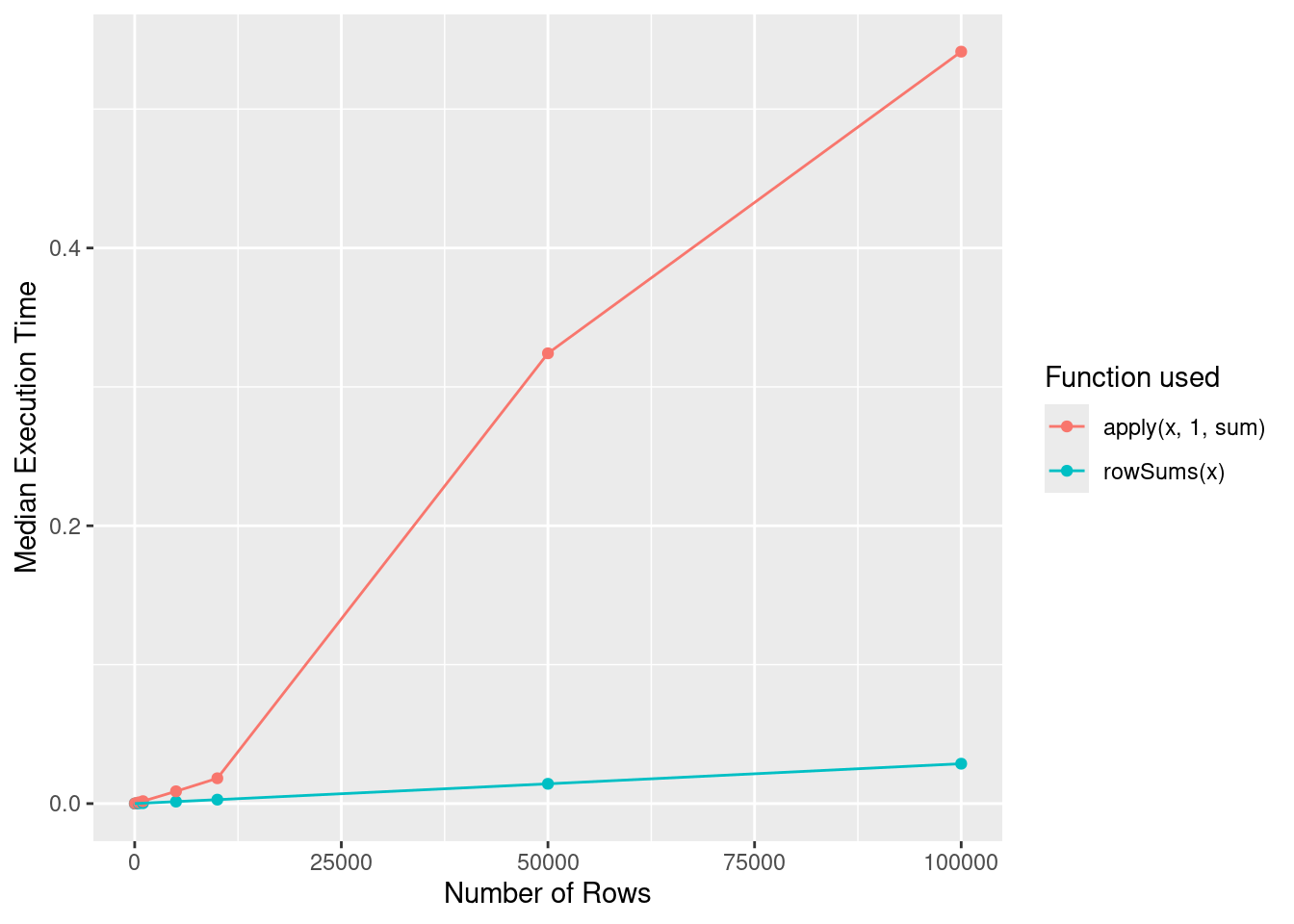
#> [6] 6.0143714 4.6147891 1.1096247 2.8759129 -0.6756857Q2. Compare the speed of apply(x, 1, sum) with rowSums(x) for varying sizes of x.
A2. We can write a custom function to vary number of rows in a matrix and extract a data frame comparing performance of these two functions.
benc_perform <- function(nRow, nCol = 100) {
  x <- matrix(data = rnorm(nRow * nCol), nrow = nRow, ncol = nCol)

  bench::mark(
    rowSums(x),
    apply(x, 1, sum)
  )[1:5]
}

nRowList <- list(10, 100, 500, 1000, 5000, 10000, 50000, 100000)

names(nRowList) <- as.character(nRowList)

benchDF <- map_dfr(
  .x = nRowList,
  .f = ~ benc_perform(.x),
  .id = "nRows"
) %>%
  mutate(nRows = as.numeric(nRows))
Plotting this data reveals that rowSums(x) has O(1) behavior, while O(n) behavior.
ggplot(
  benchDF,
  aes(
    x = as.numeric(nRows),
    y = median,
    group = as.character(expression),
    color = as.character(expression)
  )
) +
  geom_point() +
  geom_line() +
  labs(
    x = "Number of Rows",
    y = "Median Execution Time",
    colour = "Function used"
  )
Q3. How can you use crossprod() to compute a weighted sum? How much faster is it than the naive sum(x * w)?
A3. Both of these functions provide a way to compute a weighted sum:
x <- c(1:6, 2, 3)
w <- rnorm(length(x))

crossprod(x, w)[[1]]
#> [1] 15.94691
sum(x * w)[[1]]
#> [1] 15.94691
But benchmarking their performance reveals that the latter is significantly faster than the former!