10 Function factories
Attaching the needed libraries:
10.1 Factory fundamentals (Exercises 10.2.6)
Q1. The definition of force() is simple:
force
#> function (x)
#> x
#> <bytecode: 0x55e67fac4e70>
#> <environment: namespace:base>
Why is it better to force(x) instead of just x?
A1. Due to lazy evaluation, argument to a function won’t be evaluated until its value is needed. But sometimes we may want to have eager evaluation, and using force() makes this intent clearer.
Q2. Base R contains two function factories, approxfun() and ecdf(). Read their documentation and experiment to figure out what the functions do and what they return.
A2. About the two function factories-
This function factory returns a function performing the linear (or constant) interpolation.
x <- 1:10
y <- rnorm(10)
f <- approxfun(x, y)
f
#> function (v)
#> .approxfun(x, y, v, method, yleft, yright, f, na.rm)
#> <bytecode: 0x55e684f41918>
#> <environment: 0x55e684167d68>
f(x)
#>  [1] -0.7786629 -0.3894764 -2.0337983 -0.9823731  0.2478901
#>  [6] -2.1038646 -0.3814180  2.0749198  1.0271384  0.4730142
curve(f(x), 0, 11)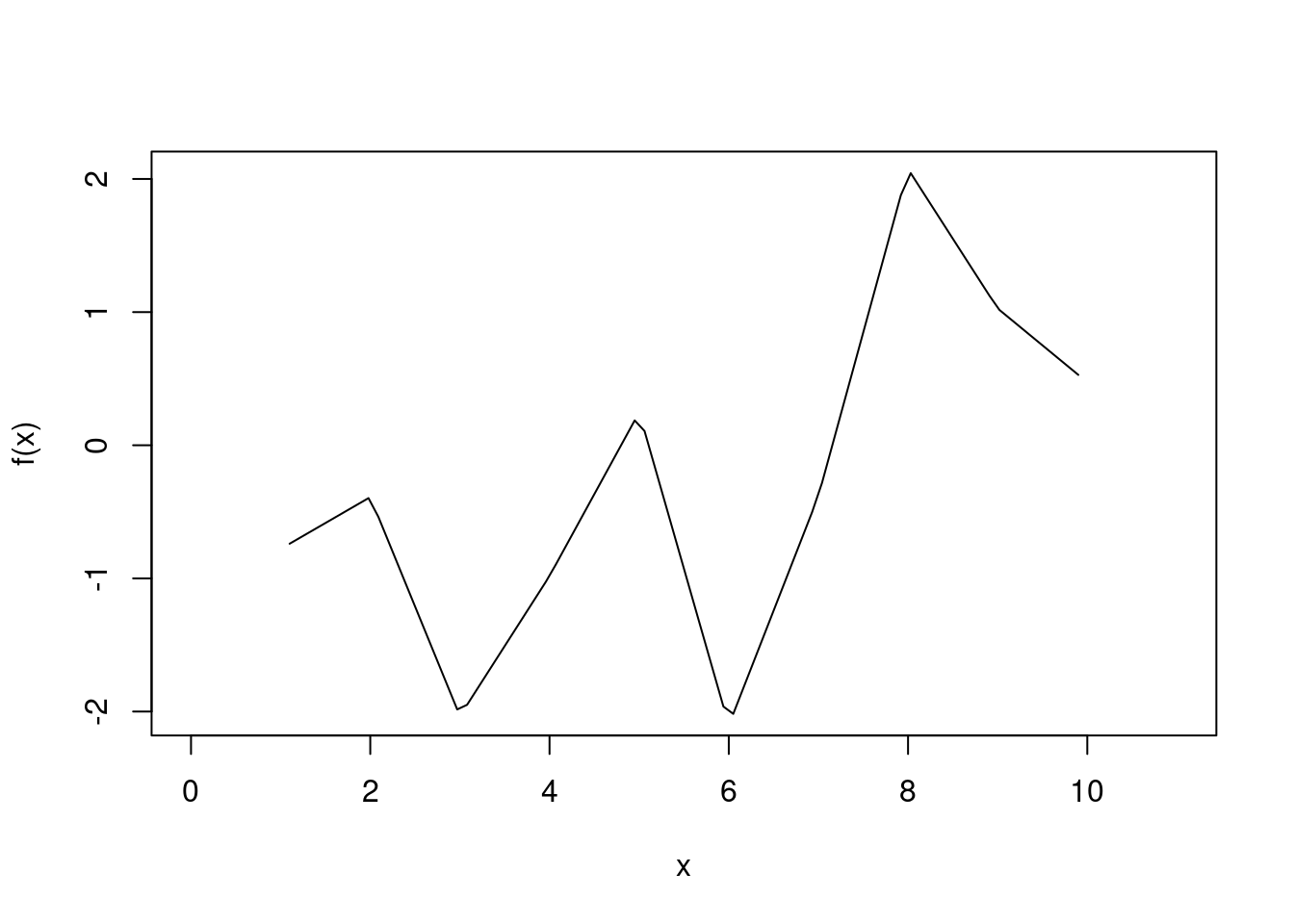
This function factory computes an empirical cumulative distribution function.
x <- rnorm(12)
f <- ecdf(x)
f
#> Empirical CDF
#> Call: ecdf(x)
#>  x[1:12] = -1.8793, -1.3221, -1.2392,  ..., 1.1604, 1.7956
f(seq(-2, 2, by = 0.1))
#>  [1] 0.00000000 0.00000000 0.08333333 0.08333333 0.08333333
#>  [6] 0.08333333 0.08333333 0.16666667 0.25000000 0.25000000
#> [11] 0.33333333 0.33333333 0.33333333 0.41666667 0.41666667
#> [16] 0.41666667 0.41666667 0.50000000 0.58333333 0.58333333
#> [21] 0.66666667 0.75000000 0.75000000 0.75000000 0.75000000
#> [26] 0.75000000 0.75000000 0.75000000 0.75000000 0.83333333
#> [31] 0.83333333 0.83333333 0.91666667 0.91666667 0.91666667
#> [36] 0.91666667 0.91666667 0.91666667 1.00000000 1.00000000
#> [41] 1.00000000
Q3. Create a function pick() that takes an index, i, as an argument and returns a function with an argument x that subsets x with i.
pick(1)(x)
# should be equivalent to
x[[1]]

lapply(mtcars, pick(5))
# should be equivalent to
lapply(mtcars, function(x) x[[5]])
A3. To write desired function, we just need to make sure that the argument i is eagerly evaluated.
pick <- function(i) {
  force(i)
  function(x) x[[i]]
}
Testing it with specified test cases:
x <- list("a", "b", "c")
identical(x[[1]], pick(1)(x))
#> [1] TRUE

identical(
  lapply(mtcars, pick(5)),
  lapply(mtcars, function(x) x[[5]])
)
#> [1] TRUE
Q4. Create a function that creates functions that compute the ithcentral moment of a numeric vector. You can test it by running the following code:
m1 <- moment(1)
m2 <- moment(2)
x <- runif(100)
stopifnot(all.equal(m1(x), 0))
stopifnot(all.equal(m2(x), var(x) * 99 / 100))
A4. The following function satisfied the specified requirements:
Testing it with specified test cases:
m1 <- moment(1)
m2 <- moment(2)
x <- runif(100)

stopifnot(all.equal(m1(x), 0))
stopifnot(all.equal(m2(x), var(x) * 99 / 100))
Q5. What happens if you don’t use a closure? Make predictions, then verify with the code below.
i <- 0
new_counter2 <- function() {
  i <<- i + 1
  i
}
A5. In case closures are not used in this context, the counts are stored in a global variable, which can be modified by other processes or even deleted.
new_counter2()
#> [1] 1

new_counter2()
#> [1] 2

new_counter2()
#> [1] 3

i <- 20
new_counter2()
#> [1] 21
Q6. What happens if you use <- instead of <<-? Make predictions, then verify with the code below.
new_counter3 <- function() {
  i <- 0
  function() {
    i <- i + 1
    i
  }
}
A6. In this case, the function will always return 1.
new_counter3()
#> function ()
#> {
#>     i <- i + 1
#>     i
#> }
#> <environment: 0x55e6875894e8>

new_counter3()
#> function ()
#> {
#>     i <- i + 1
#>     i
#> }
#> <bytecode: 0x55e687f04bd0>
#> <environment: 0x55e6875ef910>
10.2 Graphical factories (Exercises 10.3.4)
Q1. Compare and contrast ggplot2::label_bquote() with scales::number_format().
A1. To compare and contrast, let’s first look at the source code for these functions:
ggplot2::label_bquote
#> function (rows = NULL, cols = NULL, default)
#> {
#>     cols_quoted <- substitute(cols)
#>     rows_quoted <- substitute(rows)
#>     call_env <- env_parent()
#>     fun <- function(labels) {
#>         quoted <- resolve_labeller(rows_quoted, cols_quoted,
#>             labels)
#>         if (is.null(quoted)) {
#>             return(label_value(labels))
#>         }
#>         evaluate <- function(...) {
#>             params <- list(...)
#>             params <- as_environment(params, call_env)
#>             eval(substitute(bquote(expr, params), list(expr = quoted)))
#>         }
#>         list(inject(mapply(evaluate, !!!labels, SIMPLIFY = FALSE)))
#>     }
#>     structure(fun, class = "labeller")
#> }
#> <bytecode: 0x55e687b3bab8>
#> <environment: namespace:ggplot2>
scales::number_format
#> function (accuracy = NULL, scale = 1, prefix = "", suffix = "",
#>     big.mark = NULL, decimal.mark = NULL, style_positive = NULL,
#>     style_negative = NULL, scale_cut = NULL, trim = TRUE, ...)
#> {
#>     force_all(accuracy, scale, prefix, suffix, big.mark, decimal.mark,
#>         style_positive, style_negative, scale_cut, trim, ...)
#>     function(x) {
#>         number(x, accuracy = accuracy, scale = scale, prefix = prefix,
#>             suffix = suffix, big.mark = big.mark, decimal.mark = decimal.mark,
#>             style_positive = style_positive, style_negative = style_negative,
#>             scale_cut = scale_cut, trim = trim, ...)
#>     }
#> }
#> <bytecode: 0x55e687d7fad0>
#> <environment: namespace:scales>
Both of these functions return formatting functions used to style the facets labels and other labels to have the desired format in ggplot2 plots.
For example, using plotmath expression in the facet label:
library(ggplot2)

p <- ggplot(mtcars, aes(wt, mpg)) +
  geom_point()
p + facet_grid(. ~ vs, labeller = label_bquote(cols = alpha^.(vs)))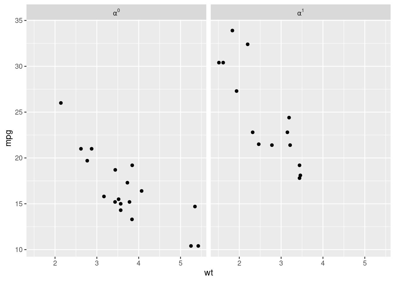
Or to display axes labels in the desired format:
library(scales)

ggplot(mtcars, aes(wt, mpg)) +
  geom_point() +
  scale_y_continuous(labels = number_format(accuracy = 0.01, decimal.mark = ","))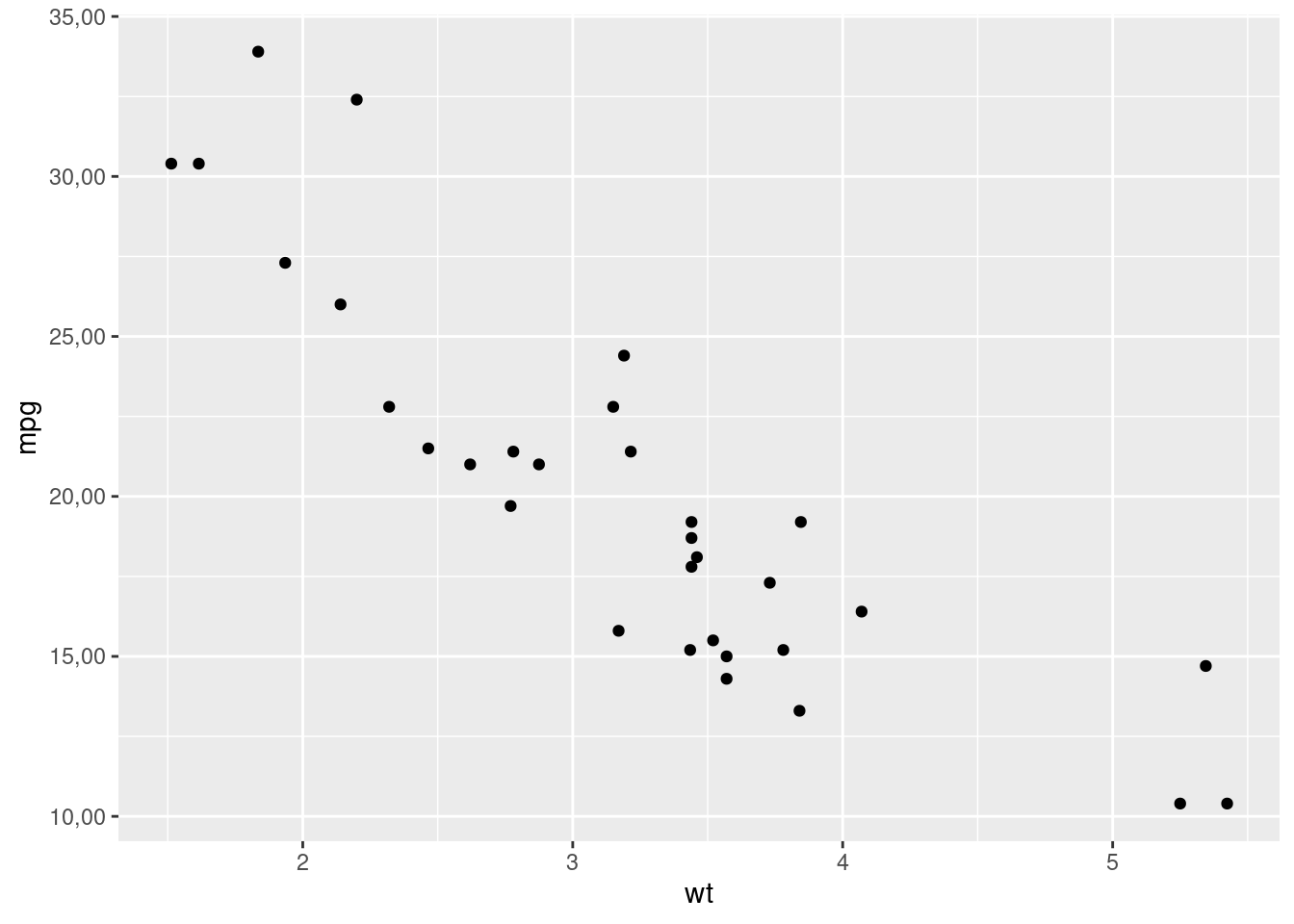
The ggplot2::label_bquote() adds an additional class to the returned function.
The scales::number_format() function is a simple pass-through method that forces evaluation of all its parameters and passes them on to the underlying scales::number() function.
10.3 Statistical factories (Exercises 10.4.4)
Q1. In boot_model(), why don’t I need to force the evaluation of df or model?
A1. We don’t need to force the evaluation of df or model because these arguments are automatically evaluated by lm():
boot_model <- function(df, formula) {
  mod <- lm(formula, data = df)
  fitted <- unname(fitted(mod))
  resid <- unname(resid(mod))
  rm(mod)

  function() {
    fitted + sample(resid)
  }
}
Q2. Why might you formulate the Box-Cox transformation like this?
boxcox3 <- function(x) {
  function(lambda) {
    if (lambda == 0) {
      log(x)
    } else {
      (x^lambda - 1) / lambda
    }
  }
}
A2. To see why we formulate this transformation like above, we can compare it to the one mentioned in the book:
boxcox2 <- function(lambda) {
  if (lambda == 0) {
    function(x) log(x)
  } else {
    function(x) (x^lambda - 1) / lambda
  }
}
Let’s have a look at one example with each:
boxcox2(1)
#> function (x)
#> (x^lambda - 1)/lambda
#> <environment: 0x55e688f799b8>

boxcox3(mtcars$wt)
#> function (lambda)
#> {
#>     if (lambda == 0) {
#>         log(x)
#>     }
#>     else {
#>         (x^lambda - 1)/lambda
#>     }
#> }
#> <environment: 0x55e6890fe240>
As can be seen:
- in
boxcox2(), we can varyxfor the same value oflambda, while - in
boxcox3(), we can varylambdafor the same vector.
Thus, boxcox3() can be handy while exploring different transformations across inputs.
Q3. Why don’t you need to worry that boot_permute() stores a copy of the data inside the function that it generates?
A3. If we look at the source code generated by the function factory, we notice that the exact data frame (mtcars) is not referenced:
boot_permute <- function(df, var) {
  n <- nrow(df)
  force(var)

  function() {
    col <- df[[var]]
    col[sample(n, replace = TRUE)]
  }
}

boot_permute(mtcars, "mpg")
#> function ()
#> {
#>     col <- df[[var]]
#>     col[sample(n, replace = TRUE)]
#> }
#> <environment: 0x55e6897e1830>
This is why we don’t need to worry about a copy being made because the df in the function environment points to the memory address of the data frame. We can confirm this by comparing their memory addresses:
boot_permute_env <- rlang::fn_env(boot_permute(mtcars, "mpg"))
rlang::env_print(boot_permute_env)
#> <environment: 0x55e689f50f58>
#> Parent: <environment: global>
#> Bindings:
#> • n: <int>
#> • df: <df[,11]>
#> • var: <chr>

identical(
  lobstr::obj_addr(boot_permute_env$df),
  lobstr::obj_addr(mtcars)
)
#> [1] TRUE
We can also check that the values of these bindings are the same as what we entered into the function factory:
identical(boot_permute_env$df, mtcars)
#> [1] TRUE
identical(boot_permute_env$var, "mpg")
#> [1] TRUE
Q4. How much time does ll_poisson2() save compared to ll_poisson1()? Use bench::mark() to see how much faster the optimisation occurs. How does changing the length of x change the results?
A4. Let’s first compare the performance of these functions with the example in the book:
ll_poisson1 <- function(x) {
  n <- length(x)

  function(lambda) {
    log(lambda) * sum(x) - n * lambda - sum(lfactorial(x))
  }
}

ll_poisson2 <- function(x) {
  n <- length(x)
  sum_x <- sum(x)
  c <- sum(lfactorial(x))

  function(lambda) {
    log(lambda) * sum_x - n * lambda - c
  }
}

x1 <- c(41, 30, 31, 38, 29, 24, 30, 29, 31, 38)

bench::mark(
  "LL1" = optimise(ll_poisson1(x1), c(0, 100), maximum = TRUE),
  "LL2" = optimise(ll_poisson2(x1), c(0, 100), maximum = TRUE)
)
#> # A tibble: 2 × 6
#>   expression      min   median `itr/sec` mem_alloc `gc/sec`
#>   <bch:expr> <bch:tm> <bch:tm>     <dbl> <bch:byt>    <dbl>
#> 1 LL1          28.7µs   30.7µs    31366.    12.8KB     15.7
#> 2 LL2          15.9µs   16.7µs    56739.        0B     11.4
As can be seen, the second version is much faster than the first version.
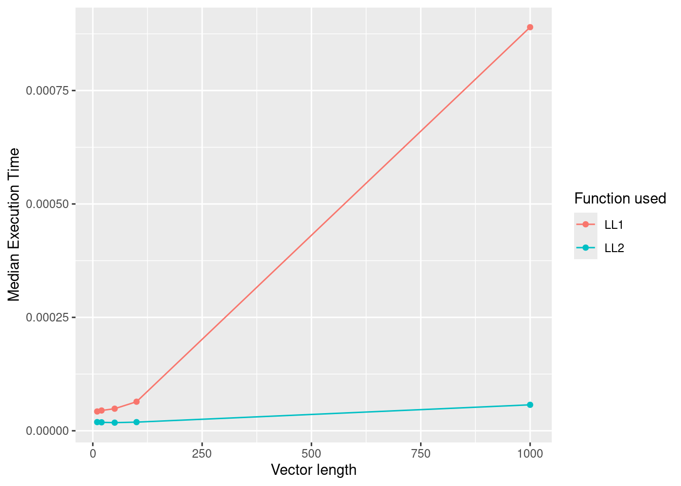
We can also vary the length of the vector and confirm that across a wide range of vector lengths, this performance advantage is observed.
generate_ll_benches <- function(n) {
  x_vec <- sample.int(n, n)

  bench::mark(
    "LL1" = optimise(ll_poisson1(x_vec), c(0, 100), maximum = TRUE),
    "LL2" = optimise(ll_poisson2(x_vec), c(0, 100), maximum = TRUE)
  )[1:4] %>%
    dplyr::mutate(length = n, .before = expression)
}

(df_bench <- purrr::map_dfr(
  .x = c(10, 20, 50, 100, 1000),
  .f = ~ generate_ll_benches(n = .x)
))
#> # A tibble: 10 × 5
#>    length expression      min   median `itr/sec`
#>     <dbl> <bch:expr> <bch:tm> <bch:tm>     <dbl>
#>  1     10 LL1          40.7µs   42.6µs    22911.
#>  2     10 LL2          18.8µs   19.7µs    49414.
#>  3     20 LL1            43µs   44.8µs    21809.
#>  4     20 LL2          18.2µs   19.2µs    50729.
#>  5     50 LL1          46.8µs   48.7µs    20130.
#>  6     50 LL2          17.4µs   18.2µs    53403.
#>  7    100 LL1          61.9µs   63.8µs    15350.
#>  8    100 LL2          18.2µs   19.3µs    49765.
#>  9   1000 LL1         831.5µs  946.3µs     1103.
#> 10   1000 LL2            56µs     58µs    16774.

ggplot(
  df_bench,
  aes(
    x = as.numeric(length),
    y = median,
    group = as.character(expression),
    color = as.character(expression)
  )
) +
  geom_point() +
  geom_line() +
  labs(
    x = "Vector length",
    y = "Median Execution Time",
    colour = "Function used"
  )
10.4 Function factories + functionals (Exercises 10.5.1)
Q1. Which of the following commands is equivalent to with(x, f(z))?
(a) `x$f(x$z)`.
(b) `f(x$z)`.
(c) `x$f(z)`.
(d) `f(z)`.
(e) It depends.
A1. It depends on whether with() is used with a data frame or a list.
f <- mean
z <- 1
x <- list(f = mean, z = 1)

identical(with(x, f(z)), x$f(x$z))
#> [1] TRUE

identical(with(x, f(z)), f(x$z))
#> [1] TRUE

identical(with(x, f(z)), x$f(z))
#> [1] TRUE

identical(with(x, f(z)), f(z))
#> [1] TRUE
Q2. Compare and contrast the effects of env_bind() vs. attach() for the following code.
A2. Let’s compare and contrast the effects of env_bind() vs. attach().
-
attach()addsfunsto the search path. Since these functions have the same names as functions in{base}package, the attached names mask the ones in the{base}package.
funs <- list(
  mean = function(x) mean(x, na.rm = TRUE),
  sum = function(x) sum(x, na.rm = TRUE)
)

attach(funs)
#> The following objects are masked from package:base:
#>
#>     mean, sum

mean
#> function (x)
#> mean(x, na.rm = TRUE)
head(search())
#> [1] ".GlobalEnv"       "funs"             "package:scales"
#> [4] "package:ggplot2"  "package:rlang"    "package:magrittr"

mean <- function(x) stop("Hi!")
mean
#> function (x)
#> stop("Hi!")
head(search())
#> [1] ".GlobalEnv"       "funs"             "package:scales"
#> [4] "package:ggplot2"  "package:rlang"    "package:magrittr"

detach(funs)-
env_bind()adds the functions infunsto the global environment, instead of masking the names in the{base}package.
env_bind(globalenv(), !!!funs)
mean
#> function (x)
#> mean(x, na.rm = TRUE)

mean <- function(x) stop("Hi!")
mean
#> function (x)
#> stop("Hi!")
env_unbind(globalenv(), names(funs))
Note that there is no "funs" in this output.
10.5 Session information
sessioninfo::session_info(include_base = TRUE)
#> ─ Session info ───────────────────────────────────────────
#>  setting  value
#>  version  R version 4.5.2 (2025-10-31)
#>  os       Ubuntu 24.04.3 LTS
#>  system   x86_64, linux-gnu
#>  ui       X11
#>  language (EN)
#>  collate  C.UTF-8
#>  ctype    C.UTF-8
#>  tz       UTC
#>  date     2026-01-13
#>  pandoc   3.8.3 @ /opt/hostedtoolcache/pandoc/3.8.3/x64/ (via rmarkdown)
#>  quarto   NA
#>
#> ─ Packages ───────────────────────────────────────────────
#>  package      * version date (UTC) lib source
#>  base         * 4.5.2   2025-10-31 [3] local
#>  bench          1.1.4   2025-01-16 [1] RSPM
#>  bookdown       0.46    2025-12-05 [1] RSPM
#>  bslib          0.9.0   2025-01-30 [1] RSPM
#>  cachem         1.1.0   2024-05-16 [1] RSPM
#>  cli            3.6.5   2025-04-23 [1] RSPM
#>  compiler       4.5.2   2025-10-31 [3] local
#>  datasets     * 4.5.2   2025-10-31 [3] local
#>  digest         0.6.39  2025-11-19 [1] RSPM
#>  downlit        0.4.5   2025-11-14 [1] RSPM
#>  dplyr          1.1.4   2023-11-17 [1] RSPM
#>  emoji          16.0.0  2024-10-28 [1] RSPM
#>  evaluate       1.0.5   2025-08-27 [1] RSPM
#>  farver         2.1.2   2024-05-13 [1] RSPM
#>  fastmap        1.2.0   2024-05-15 [1] RSPM
#>  fs             1.6.6   2025-04-12 [1] RSPM
#>  generics       0.1.4   2025-05-09 [1] RSPM
#>  ggplot2      * 4.0.1   2025-11-14 [1] RSPM
#>  glue           1.8.0   2024-09-30 [1] RSPM
#>  graphics     * 4.5.2   2025-10-31 [3] local
#>  grDevices    * 4.5.2   2025-10-31 [3] local
#>  grid           4.5.2   2025-10-31 [3] local
#>  gtable         0.3.6   2024-10-25 [1] RSPM
#>  htmltools      0.5.9   2025-12-04 [1] RSPM
#>  jquerylib      0.1.4   2021-04-26 [1] RSPM
#>  jsonlite       2.0.0   2025-03-27 [1] RSPM
#>  knitr          1.51    2025-12-20 [1] RSPM
#>  labeling       0.4.3   2023-08-29 [1] RSPM
#>  lifecycle      1.0.5   2026-01-08 [1] RSPM
#>  lobstr         1.1.3   2025-11-14 [1] RSPM
#>  magrittr     * 2.0.4   2025-09-12 [1] RSPM
#>  memoise        2.0.1   2021-11-26 [1] RSPM
#>  methods      * 4.5.2   2025-10-31 [3] local
#>  pillar         1.11.1  2025-09-17 [1] RSPM
#>  pkgconfig      2.0.3   2019-09-22 [1] RSPM
#>  profmem        0.7.0   2025-05-02 [1] RSPM
#>  purrr          1.2.1   2026-01-09 [1] RSPM
#>  R6             2.6.1   2025-02-15 [1] RSPM
#>  RColorBrewer   1.1-3   2022-04-03 [1] RSPM
#>  rlang        * 1.1.7   2026-01-09 [1] RSPM
#>  rmarkdown      2.30    2025-09-28 [1] RSPM
#>  S7             0.2.1   2025-11-14 [1] RSPM
#>  sass           0.4.10  2025-04-11 [1] RSPM
#>  scales       * 1.4.0   2025-04-24 [1] RSPM
#>  sessioninfo    1.2.3   2025-02-05 [1] RSPM
#>  stats        * 4.5.2   2025-10-31 [3] local
#>  stringi        1.8.7   2025-03-27 [1] RSPM
#>  stringr        1.6.0   2025-11-04 [1] RSPM
#>  tibble         3.3.1   2026-01-11 [1] RSPM
#>  tidyselect     1.2.1   2024-03-11 [1] RSPM
#>  tools          4.5.2   2025-10-31 [3] local
#>  utf8           1.2.6   2025-06-08 [1] RSPM
#>  utils        * 4.5.2   2025-10-31 [3] local
#>  vctrs          0.6.5   2023-12-01 [1] RSPM
#>  withr          3.0.2   2024-10-28 [1] RSPM
#>  xfun           0.55    2025-12-16 [1] RSPM
#>  xml2           1.5.1   2025-12-01 [1] RSPM
#>  yaml           2.3.12  2025-12-10 [1] RSPM
#>
#>  [1] /home/runner/work/_temp/Library
#>  [2] /opt/R/4.5.2/lib/R/site-library
#>  [3] /opt/R/4.5.2/lib/R/library
#>  * ── Packages attached to the search path.
#>
#> ──────────────────────────────────────────────────────────