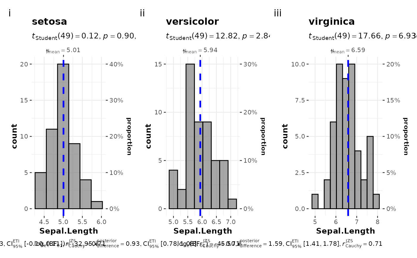
Grouped histograms for distribution of a numeric variable

Helper function for ggstatsplot::gghistostats to apply this function across multiple levels of a given factor and combining the resulting plots using ggstatsplot::combine_plots.

Usage

grouped_gghistostats(
  data,
  x,
  grouping.var,
  binwidth = NULL,
  plotgrid.args = list(),
  annotation.args = list(),
  ...
)

Arguments

data

A data frame (or a tibble) from which variables specified are to be taken. Other data types (e.g., matrix,table, array, etc.) will not be accepted. Additionally, grouped data frames from {dplyr} should be ungrouped before they are entered as data.

x

A numeric variable from the data frame data.

grouping.var

A single grouping variable.

binwidth

The width of the histogram bins. Can be specified as a numeric value, or a function that calculates width from x. The default is to use the max(x) - min(x) / sqrt(N). You should always check this value and explore multiple widths to find the best to illustrate the stories in your data.

plotgrid.args

A list of additional arguments passed to patchwork::wrap_plots(), except for guides argument which is already separately specified here.

annotation.args

A list of additional arguments passed to patchwork::plot_annotation().

...

Arguments passed on to gghistostats

normal.curve

A logical value that decides whether to super-impose a normal curve using stats::dnorm(mean(x), stats::sd(x)). Default is FALSE.

normal.curve.args

A list of additional aesthetic arguments to be passed to the normal curve.

bin.args

A list of additional aesthetic arguments to be passed to the stat_bin used to display the bins. Do not specify binwidth argument in this list since it has already been specified using the dedicated argument.

centrality.line.args

A list of additional aesthetic arguments to be passed to the geom_line used to display the lines corresponding to the centrality parameter.

type

A character specifying the type of statistical approach:

"parametric"
"nonparametric"
"robust"
"bayes"

You can specify just the initial letter.

test.value

A number indicating the true value of the mean (Default: 0).

digits

Number of digits for rounding or significant figures. May also be "signif" to return significant figures or "scientific" to return scientific notation. Control the number of digits by adding the value as suffix, e.g. digits = "scientific4" to have scientific notation with 4 decimal places, or digits = "signif5" for 5 significant figures (see also signif()).

conf.level

Scalar between 0 and 1 (default: 95% confidence/credible intervals, 0.95). If NULL, no confidence intervals will be computed.

tr

Trim level for the mean when carrying out robust tests. In case of an error, try reducing the value of tr, which is by default set to 0.2. Lowering the value might help.

bf.prior

A number between 0.5 and 2 (default 0.707), the prior width to use in calculating Bayes factors and posterior estimates. In addition to numeric arguments, several named values are also recognized: "medium", "wide", and "ultrawide", corresponding to r scale values of 1/2, sqrt(2)/2, and 1, respectively. In case of an ANOVA, this value corresponds to scale for fixed effects.

effsize.type

Type of effect size needed for parametric tests. The argument can be "d" (for Cohen's d) or "g" (for Hedge's g).

xlab

Label for x axis variable. If NULL (default), variable name for x will be used.

bf.message

Logical that decides whether to display Bayes Factor in favor of the null hypothesis. This argument is relevant only for parametric test (Default: TRUE).

results.subtitle

Decides whether the results of statistical tests are to be displayed as a subtitle (Default: TRUE). If set to FALSE, only the plot will be returned.

subtitle

The text for the plot subtitle. Will work only if results.subtitle = FALSE.

caption

The text for the plot caption. This argument is relevant only if bf.message = FALSE.

centrality.plotting

Logical that decides whether centrality tendency measure is to be displayed as a point with a label (Default: TRUE). Function decides which central tendency measure to show depending on the type argument.

mean for parametric statistics
median for non-parametric statistics
trimmed mean for robust statistics
MAP estimator for Bayesian statistics

If you want default centrality parameter, you can specify this using centrality.type argument.

centrality.type

Decides which centrality parameter is to be displayed. The default is to choose the same as type argument. You can specify this to be:

"parameteric" (for mean)
"nonparametric" (for median)
robust (for trimmed mean)
bayes (for MAP estimator)

Just as type argument, abbreviations are also accepted.

ggplot.component

A ggplot component to be added to the plot prepared by {ggstatsplot}. This argument is primarily helpful for grouped_ variants of all primary functions. Default is NULL. The argument should be entered as a {ggplot2} function or a list of {ggplot2} functions.

ggtheme

A {ggplot2} theme. Default value is ggstatsplot::theme_ggstatsplot(). Any of the {ggplot2} themes (e.g., theme_bw()), or themes from extension packages are allowed (e.g., ggthemes::theme_fivethirtyeight(), hrbrthemes::theme_ipsum_ps(), etc.). But note that sometimes these themes will remove some of the details that {ggstatsplot} plots typically contains. For example, if relevant, ggbetweenstats() shows details about multiple comparison test as a label on the secondary Y-axis. Some themes (e.g. ggthemes::theme_fivethirtyeight()) will remove the secondary Y-axis and thus the details as well.

Details

For details, see: https://indrajeetpatil.github.io/ggstatsplot/articles/web_only/gghistostats.html

Examples

# for reproducibility
set.seed(123)

# plot
grouped_gghistostats(
  data            = iris,
  x               = Sepal.Length,
  test.value      = 5,
  grouping.var    = Species,
  plotgrid.args   = list(nrow = 1),
  annotation.args = list(tag_levels = "i")
)

Usage

Arguments

Details

See also

Examples