Scatterplot with marginal distributions and statistical results

Scatterplots from {ggplot2} combined with marginal densigram (density + histogram) plots with statistical details.

Usage

ggscatterstats(
  data,
  x,
  y,
  type = "parametric",
  conf.level = 0.95,
  bf.prior = 0.707,
  bf.message = TRUE,
  tr = 0.2,
  digits = 2L,
  results.subtitle = TRUE,
  label.var = NULL,
  label.expression = NULL,
  marginal = TRUE,
  point.args = list(size = 3, alpha = 0.4, stroke = 0),
  point.width.jitter = 0,
  point.height.jitter = 0,
  point.label.args = list(size = 3, max.overlaps = 1e+06),
  smooth.line.args = list(linewidth = 1.5, color = "blue", method = "lm", formula = y ~
    x),
  xsidehistogram.args = list(fill = "#009E73", color = "black", na.rm = TRUE),
  ysidehistogram.args = list(fill = "#D55E00", color = "black", na.rm = TRUE),
  xlab = NULL,
  ylab = NULL,
  title = NULL,
  subtitle = NULL,
  caption = NULL,
  ggtheme = ggstatsplot::theme_ggstatsplot(),
  ggplot.component = NULL,
  ...
)

Arguments

data

A data frame (or a tibble) from which variables specified are to be taken. Other data types (e.g., matrix,table, array, etc.) will not be accepted. Additionally, grouped data frames from {dplyr} should be ungrouped before they are entered as data.

x

The column in data containing the explanatory variable to be plotted on the x-axis.

y

The column in data containing the response (outcome) variable to be plotted on the y-axis.

type

A character specifying the type of statistical approach:

"parametric"
"nonparametric"
"robust"
"bayes"

You can specify just the initial letter.

conf.level

Scalar between 0 and 1 (default: 95% confidence/credible intervals, 0.95). If NULL, no confidence intervals will be computed.

bf.prior

A number between 0.5 and 2 (default 0.707), the prior width to use in calculating Bayes factors and posterior estimates. In addition to numeric arguments, several named values are also recognized: "medium", "wide", and "ultrawide", corresponding to r scale values of 1/2, sqrt(2)/2, and 1, respectively. In case of an ANOVA, this value corresponds to scale for fixed effects.

bf.message

Logical that decides whether to display Bayes Factor in favor of the null hypothesis. This argument is relevant only for parametric test (Default: TRUE).

tr

Trim level for the mean when carrying out robust tests. In case of an error, try reducing the value of tr, which is by default set to 0.2. Lowering the value might help.

digits

Number of digits for rounding or significant figures. May also be "signif" to return significant figures or "scientific" to return scientific notation. Control the number of digits by adding the value as suffix, e.g. digits = "scientific4" to have scientific notation with 4 decimal places, or digits = "signif5" for 5 significant figures (see also signif()).

results.subtitle

Decides whether the results of statistical tests are to be displayed as a subtitle (Default: TRUE). If set to FALSE, only the plot will be returned.

label.var

Variable to use for points labels entered as a symbol (e.g. var1).

label.expression

An expression evaluating to a logical vector that determines the subset of data points to label (e.g. y < 4 & z < 20). While using this argument with purrr::pmap(), you will have to provide a quoted expression (e.g. quote(y < 4 & z < 20)).

marginal

Decides whether marginal distributions will be plotted on axes using ggside functions. The default is TRUE. The package ggside must already be installed by the user.

point.args

A list of additional aesthetic arguments to be passed to geom_point geom used to display the raw data points.

point.width.jitter, point.height.jitter

Degree of jitter in x and y direction, respectively. Defaults to 0 (0%) of the resolution of the data. Note that the jitter should not be specified in the point.args because this information will be passed to two different geoms: one displaying the points and the other displaying the *labels for these points.

point.label.args

A list of additional aesthetic arguments to be passed to ggrepel::geom_label_repel geom used to display the labels.

smooth.line.args

A list of additional aesthetic arguments to be passed to geom_smooth geom used to display the regression line.

xsidehistogram.args, ysidehistogram.args

A list of arguments passed to respective geom_s from the {ggside} package to change the marginal distribution histograms plots.

xlab

Label for x axis variable. If NULL (default), variable name for x will be used.

ylab

Labels for y axis variable. If NULL (default), variable name for y will be used.

title

The text for the plot title.

subtitle

The text for the plot subtitle. Will work only if results.subtitle = FALSE.

caption

The text for the plot caption. This argument is relevant only if bf.message = FALSE.

ggtheme

A {ggplot2} theme. Default value is ggstatsplot::theme_ggstatsplot(). Any of the {ggplot2} themes (e.g., theme_bw()), or themes from extension packages are allowed (e.g., ggthemes::theme_fivethirtyeight(), hrbrthemes::theme_ipsum_ps(), etc.). But note that sometimes these themes will remove some of the details that {ggstatsplot} plots typically contains. For example, if relevant, ggbetweenstats() shows details about multiple comparison test as a label on the secondary Y-axis. Some themes (e.g. ggthemes::theme_fivethirtyeight()) will remove the secondary Y-axis and thus the details as well.

ggplot.component

A ggplot component to be added to the plot prepared by {ggstatsplot}. This argument is primarily helpful for grouped_ variants of all primary functions. Default is NULL. The argument should be entered as a {ggplot2} function or a list of {ggplot2} functions.

...

Currently ignored.

Details

For details, see: https://indrajeetpatil.github.io/ggstatsplot/articles/web_only/ggscatterstats.html

Note

The plot uses ggrepel::geom_label_repel() to attempt to keep labels from over-lapping to the largest degree possible. As a consequence plot times will slow down massively (and the plot file will grow in size) if you have a lot of labels that overlap.

Summary of graphics

graphical element	`geom` used	argument for further modification
histogram bin	`ggplot2::stat_bin()`	`bin.args`
centrality measure line	`ggplot2::geom_vline()`	`centrality.line.args`
normality curve	`ggplot2::stat_function()`	`normal.curve.args`

Correlation analyses

The table below provides summary about:

statistical test carried out for inferential statistics
type of effect size estimate and a measure of uncertainty for this estimate
functions used internally to compute these details

Hypothesis testing and Effect size estimation

Type	Test	CI available?	Function used
Parametric	Pearson's correlation coefficient	Yes	`correlation::correlation()`
Non-parametric	Spearman's rank correlation coefficient	Yes	`correlation::correlation()`
Robust	Winsorized Pearson's correlation coefficient	Yes	`correlation::correlation()`
Bayesian	Bayesian Pearson's correlation coefficient	Yes	`correlation::correlation()`

Examples

set.seed(123)

# creating a plot
p <- ggscatterstats(
  iris,
  x = Sepal.Width,
  y = Petal.Length,
  label.var = Species,
  label.expression = Sepal.Length > 7.6
) +
  ggplot2::geom_rug(sides = "b")
#> Registered S3 method overwritten by 'ggside':
#>   method from   
#>   +.gg   ggplot2

# looking at the plot
p
#> `stat_xsidebin()` using `bins = 30`. Pick better value with `binwidth`.
#> `stat_ysidebin()` using `bins = 30`. Pick better value with `binwidth`.


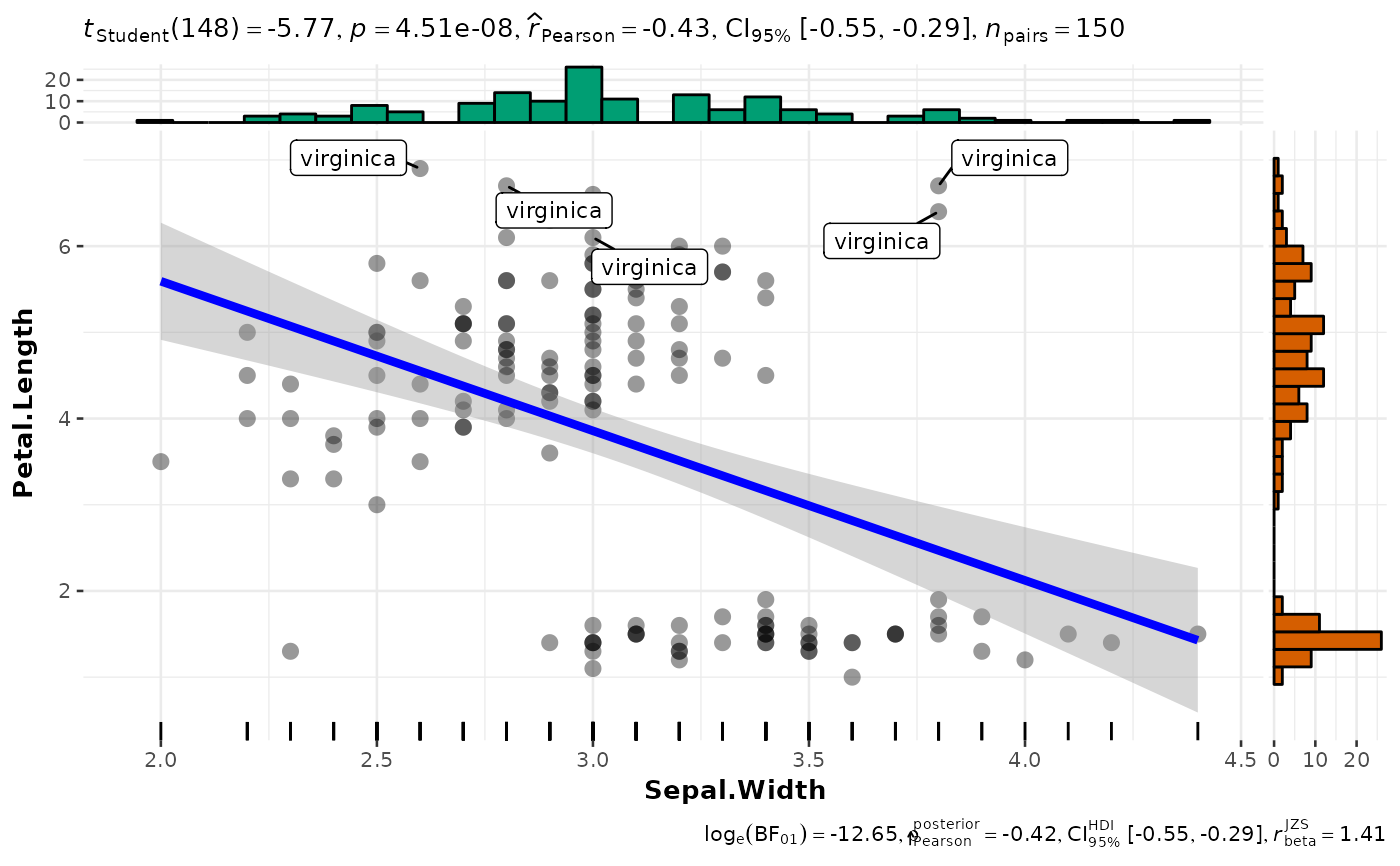# extracting details from statistical tests
extract_stats(p)
#> $subtitle_data
#> # A tibble: 1 × 14
#>   parameter1  parameter2   effectsize          estimate conf.level conf.low
#>   <chr>       <chr>        <chr>                  <dbl>      <dbl>    <dbl>
#> 1 Sepal.Width Petal.Length Pearson correlation   -0.428       0.95   -0.551
#>   conf.high statistic df.error      p.value method              n.obs
#>       <dbl>     <dbl>    <int>        <dbl> <chr>               <int>
#> 1    -0.288     -5.77      148 0.0000000451 Pearson correlation   150
#>   conf.method expression
#>   <chr>       <list>    
#> 1 normal      <language>
#> 
#> $caption_data
#> # A tibble: 1 × 17
#>   parameter1  parameter2   effectsize                   estimate conf.level
#>   <chr>       <chr>        <chr>                           <dbl>      <dbl>
#> 1 Sepal.Width Petal.Length Bayesian Pearson correlation   -0.422       0.95
#>   conf.low conf.high    pd rope.percentage prior.distribution prior.location
#>      <dbl>     <dbl> <dbl>           <dbl> <chr>                       <dbl>
#> 1   -0.551    -0.290     1               0 beta                         1.41
#>   prior.scale    bf10 method                       n.obs conf.method expression
#>         <dbl>   <dbl> <chr>                        <int> <chr>       <list>    
#> 1        1.41 312665. Bayesian Pearson correlation   150 HDI         <language>
#> 
#> $pairwise_comparisons_data
#> NULL
#> 
#> $descriptive_data
#> NULL
#> 
#> $one_sample_data
#> NULL
#> 
#> $tidy_data
#> NULL
#> 
#> $glance_data
#> NULL
#>