Dot plot/chart for labeled numeric data.

A dot chart (as described by William S. Cleveland) with statistical details from one-sample test.

Usage

ggdotplotstats(
  data,
  x,
  y,
  xlab = NULL,
  ylab = NULL,
  title = NULL,
  subtitle = NULL,
  caption = NULL,
  type = "parametric",
  test.value = 0,
  bf.prior = 0.707,
  bf.message = TRUE,
  effsize.type = "g",
  conf.level = 0.95,
  tr = 0.2,
  digits = 2L,
  results.subtitle = TRUE,
  point.args = list(color = "black", size = 3, shape = 16),
  centrality.plotting = TRUE,
  centrality.type = type,
  centrality.line.args = list(color = "blue", linewidth = 1, linetype = "dashed"),
  ggplot.component = NULL,
  ggtheme = ggstatsplot::theme_ggstatsplot(),
  ...
)

Arguments

data

A data frame (or a tibble) from which variables specified are to be taken. Other data types (e.g., matrix,table, array, etc.) will not be accepted. Additionally, grouped data frames from {dplyr} should be ungrouped before they are entered as data.

x

A numeric variable from the data frame data.

y

Label or grouping variable.

xlab

Label for x axis variable. If NULL (default), variable name for x will be used.

ylab

Labels for y axis variable. If NULL (default), variable name for y will be used.

title

The text for the plot title.

subtitle

The text for the plot subtitle. Will work only if results.subtitle = FALSE.

caption

The text for the plot caption. This argument is relevant only if bf.message = FALSE.

type

A character specifying the type of statistical approach:

"parametric"
"nonparametric"
"robust"
"bayes"

You can specify just the initial letter.

test.value

A number indicating the true value of the mean (Default: 0).

bf.prior

A number between 0.5 and 2 (default 0.707), the prior width to use in calculating Bayes factors and posterior estimates. In addition to numeric arguments, several named values are also recognized: "medium", "wide", and "ultrawide", corresponding to r scale values of 1/2, sqrt(2)/2, and 1, respectively. In case of an ANOVA, this value corresponds to scale for fixed effects.

bf.message

Logical that decides whether to display Bayes Factor in favor of the null hypothesis. This argument is relevant only for parametric test (Default: TRUE).

effsize.type

Type of effect size needed for parametric tests. The argument can be "d" (for Cohen's d) or "g" (for Hedge's g).

conf.level

Scalar between 0 and 1 (default: 95% confidence/credible intervals, 0.95). If NULL, no confidence intervals will be computed.

tr

Trim level for the mean when carrying out robust tests. In case of an error, try reducing the value of tr, which is by default set to 0.2. Lowering the value might help.

digits

Number of digits for rounding or significant figures. May also be "signif" to return significant figures or "scientific" to return scientific notation. Control the number of digits by adding the value as suffix, e.g. digits = "scientific4" to have scientific notation with 4 decimal places, or digits = "signif5" for 5 significant figures (see also signif()).

results.subtitle

Decides whether the results of statistical tests are to be displayed as a subtitle (Default: TRUE). If set to FALSE, only the plot will be returned.

point.args

A list of additional aesthetic arguments passed to geom_point.

centrality.plotting

Logical that decides whether centrality tendency measure is to be displayed as a point with a label (Default: TRUE). Function decides which central tendency measure to show depending on the type argument.

mean for parametric statistics
median for non-parametric statistics
trimmed mean for robust statistics
MAP estimator for Bayesian statistics

If you want default centrality parameter, you can specify this using centrality.type argument.

centrality.type

Decides which centrality parameter is to be displayed. The default is to choose the same as type argument. You can specify this to be:

"parameteric" (for mean)
"nonparametric" (for median)
robust (for trimmed mean)
bayes (for MAP estimator)

Just as type argument, abbreviations are also accepted.

centrality.line.args

A list of additional aesthetic arguments to be passed to the geom_line used to display the lines corresponding to the centrality parameter.

ggplot.component

A ggplot component to be added to the plot prepared by {ggstatsplot}. This argument is primarily helpful for grouped_ variants of all primary functions. Default is NULL. The argument should be entered as a {ggplot2} function or a list of {ggplot2} functions.

ggtheme

A {ggplot2} theme. Default value is ggstatsplot::theme_ggstatsplot(). Any of the {ggplot2} themes (e.g., theme_bw()), or themes from extension packages are allowed (e.g., ggthemes::theme_fivethirtyeight(), hrbrthemes::theme_ipsum_ps(), etc.). But note that sometimes these themes will remove some of the details that {ggstatsplot} plots typically contains. For example, if relevant, ggbetweenstats() shows details about multiple comparison test as a label on the secondary Y-axis. Some themes (e.g. ggthemes::theme_fivethirtyeight()) will remove the secondary Y-axis and thus the details as well.

...

Currently ignored.

Details

For details, see: https://indrajeetpatil.github.io/ggstatsplot/articles/web_only/ggdotplotstats.html

Summary of graphics

graphical element	`geom` used	argument for further modification
histogram bin	`ggplot2::stat_bin()`	`bin.args`
centrality measure line	`ggplot2::geom_vline()`	`centrality.line.args`
normality curve	`ggplot2::stat_function()`	`normal.curve.args`

One-sample tests

The table below provides summary about:

statistical test carried out for inferential statistics
type of effect size estimate and a measure of uncertainty for this estimate
functions used internally to compute these details

Hypothesis testing

Type	Test	Function used
Parametric	One-sample Student's t-test	`stats::t.test()`
Non-parametric	One-sample Wilcoxon test	`stats::wilcox.test()`
Robust	Bootstrap-t method for one-sample test	`WRS2::trimcibt()`
Bayesian	One-sample Student's t-test	`BayesFactor::ttestBF()`

Effect size estimation

Type	Effect size	CI available?	Function used
Parametric	Cohen's d, Hedge's g	Yes	`effectsize::cohens_d()`, `effectsize::hedges_g()`
Non-parametric	r (rank-biserial correlation)	Yes	`effectsize::rank_biserial()`
Robust	trimmed mean	Yes	`WRS2::trimcibt()`
Bayes Factor	difference	Yes	`bayestestR::describe_posterior()`

Examples

# for reproducibility
set.seed(123)

# creating a plot
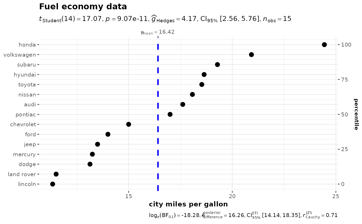
p <- ggdotplotstats(
  data = ggplot2::mpg,
  x = cty,
  y = manufacturer,
  title = "Fuel economy data",
  xlab = "city miles per gallon"
)

# looking at the plot
p


# extracting details from statistical tests
extract_stats(p)
#> $subtitle_data
#> # A tibble: 1 × 15
#>      mu statistic df.error  p.value method            alternative effectsize
#>   <dbl>     <dbl>    <dbl>    <dbl> <chr>             <chr>       <chr>     
#> 1     0      17.1       14 9.07e-11 One Sample t-test two.sided   Hedges' g 
#>   estimate conf.level conf.low conf.high conf.method conf.distribution n.obs
#>      <dbl>      <dbl>    <dbl>     <dbl> <chr>       <chr>             <int>
#> 1     4.17       0.95     2.56      5.76 ncp         t                    15
#>   expression
#>   <list>    
#> 1 <language>
#> 
#> $caption_data
#> # A tibble: 1 × 16
#>   term       effectsize      estimate conf.level conf.low conf.high    pd
#>   <chr>      <chr>              <dbl>      <dbl>    <dbl>     <dbl> <dbl>
#> 1 Difference Bayesian t-test     16.3       0.95     14.1      18.4     1
#>   prior.distribution prior.location prior.scale      bf10 method         
#>   <chr>                       <dbl>       <dbl>     <dbl> <chr>          
#> 1 cauchy                          0       0.707 87122783. Bayesian t-test
#>   conf.method log_e_bf10 n.obs expression
#>   <chr>            <dbl> <int> <list>    
#> 1 ETI               18.3    15 <language>
#> 
#> $pairwise_comparisons_data
#> NULL
#> 
#> $descriptive_data
#> NULL
#> 
#> $one_sample_data
#> NULL
#> 
#> $tidy_data
#> NULL
#> 
#> $glance_data
#> NULL
#>